２原子分子の分子軌道のLCAO近似を可視化する

Introduction

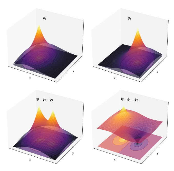
２原子分子の分子軌道 $\Psi$ を既知の関数（原子軌道など）の線形結合で表すというLCAO近似を分かりやすく表したい $$ \Psi = c_1 \phi_1 + c_2 \phi_2$$
とくに、展開係数 ${c_n}$ の値を変えるだけで、分子関数$\Psi$のカタチが違うんだよということを分かりやすくしたい

Results

スレーター型関数の線形結合

import numpy as np
import matplotlib.pyplot as plt
from mpl_toolkits.mplot3d import Axes3D

# Define the Slater-type function
def slater(r, coeff, alpha):
    return coeff * np.exp(-alpha * r)

# Define the range and grid
x_values = np.linspace(-3, 3, 400)
x_grid, y_grid = np.meshgrid(x_values, np.linspace(-2, 2, 400))
center1 = -1
center2 = 1

# Parameters for the Slater-type functions
alpha1 = 1
alpha2 = 1
coeff1 = 1
coeff2 = 1

# Scenarios for plotting
scenarios = [
    (coeff1, 0, r'$\phi_1$'),
    (0, coeff2, r'$\phi_2$'),
    (coeff1, coeff2, r'$\Psi = \phi_1 + \phi_2$'),
    (coeff1, -coeff2, r'$\Psi = \phi_1 - \phi_2$')
]

# Create a new figure for 3D plotting with adjusted axis label positions
fig = plt.figure(figsize=(15, 12))

for i, (coeff1_scenario, coeff2_scenario, title) in enumerate(scenarios):
    # Create a subplot for the current scenario
    ax = fig.add_subplot(2, 2, i+1, projection='3d')
    
    # Calculate the distance from each center
    r1 = np.sqrt((x_grid - center1)**2 + y_grid**2)
    r2 = np.sqrt((x_grid - center2)**2 + y_grid**2)
    
    # Compute the values for the combined Slater-type functions
    z1 = slater(r1, coeff1_scenario, alpha1)
    z2 = slater(r2, coeff2_scenario, alpha2)
    z_combined = z1 + z2
    
    # Plot the 3D surface
    ax.plot_surface(x_grid, y_grid, z_combined, cmap='inferno', edgecolor='none', alpha=0.8)

    # Plot the 2D heatmap at the bottom
    ax.contourf(x_grid, y_grid, z_combined, zdir='z', offset=z_combined.min(), cmap='inferno', alpha=0.6)

    # Set labels with adjusted positions and title
    ax.set_xlabel('x', labelpad=-10)
    ax.set_ylabel('y', labelpad=-10)
    ax.set_title(title, y=0.85)

    # Remove the tick labels
    ax.set_xticks([])
    ax.set_yticks([])
    ax.set_zticks([])

# Adjust the layout to maintain reduced spaces between subplots
plt.subplots_adjust(wspace=-0.35, hspace=-0.05)

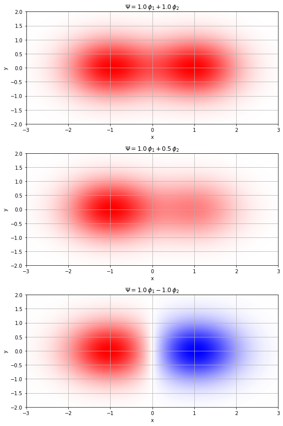
plt.show()

ガウス型関数の線形結合（横から見た図）

import numpy as np
import matplotlib.pyplot as plt
from matplotlib.colors import LinearSegmentedColormap

# Define the Gaussian functions centered at two different atoms
def gaussian(x, center, coeff, width):
    return coeff * np.exp(-width * (x - center)**2)

# Parameters for the Gaussian functions
center1 = -1
center2 = 1
width = 1
x_values = np.linspace(-3, 3, 400)
x_grid, y_grid = np.meshgrid(x_values, np.linspace(-2, 2, 400))

# Custom colormap
cm = LinearSegmentedColormap.from_list('custom_density', [(0, 0, 1), (1, 1, 1), (1, 0, 0)], N=256)

# Define the coefficients and phase for each scenario
coeffs_scenarios = [
    (1, 1, r'$\Psi = 1.0 \, \phi_1 + 1.0 \, \phi_2$'),
    (1, 0.5, r'$\Psi = 1.0 \, \phi_1 + 0.5 \, \phi_2$'),
    (1, -1, r'$\Psi = 1.0 \, \phi_1 - 1.0 \, \phi_2$')
]

# Plotting
fig, axs = plt.subplots(len(coeffs_scenarios), 1, figsize=(8, 12))

for i, (coeff1_scenario, coeff2_scenario, title) in enumerate(coeffs_scenarios):
    z1 = gaussian(x_grid, center1, coeff1_scenario, width) * np.exp(-width * (y_grid**2))
    z2 = gaussian(x_grid, center2, coeff2_scenario, width) * np.exp(-width * (y_grid**2))
    z_combined = z1 + z2

    max_abs_combined = np.max(np.abs(z_combined))
    im = axs[i].imshow(z_combined, extent=[x_values.min(), x_values.max(), -2, 2], 
                       aspect='auto', origin='lower', vmin=-max_abs_combined, vmax=max_abs_combined, cmap=cm)
    axs[i].set_title(title)
    axs[i].set_xlabel('x')
    axs[i].set_ylabel('y')
    axs[i].grid(True)

# Adjust spacing
fig.tight_layout()

plt.show()

Conclusion

できた

量子化学教育

Posted : 23.10.25