スレーター型基底 vs ガウス型基底：可視化して比較

Introduction

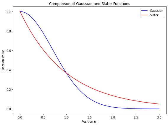
量子化学計算で用いる基底関数について、スレーター型関数 $\exp(-\zeta r)$ とガウス型関数 $\exp(-\alpha r^2)$を可視化して比較したい
ガウス型関数については、いくつかを線形結合させた短縮型ガウス基底についても、スレーター型関数と比較したい

Results

スレーター型基底 vs ガウス型基底

import numpy as np
import matplotlib.pyplot as plt

# Define Gaussian and Slater functions
def gaussian(r, coeff, alpha):
    return coeff * np.exp(-alpha * r**2)

def slater(r, coeff, alpha):
    return coeff * np.exp(-alpha * r)

# Define the range for plotting
r_values = np.linspace(0, 3, 400)

# Parameters for the functions (based on the reference image and typical values)
alpha_gaussian = 1
alpha_slater = 1
coeff = 1

# Compute the values for Gaussian and Slater functions
gaussian_values = gaussian(r_values, coeff, alpha_gaussian)
slater_values = slater(r_values, coeff, alpha_slater)

# Plotting
fig, ax = plt.subplots(figsize=(8, 6))

ax.plot(r_values, gaussian_values, label="Gaussian", color="blue", linestyle="-")
ax.plot(r_values, slater_values, label="Slater", color="red", linestyle="-")

ax.set_xlabel("Position (r)")
ax.set_ylabel("Function Value")
ax.legend()
ax.set_title("Comparison of Gaussian and Slater Functions")

plt.tight_layout()
plt.show()

スレーター型基底 vs 短縮ガウス型基底

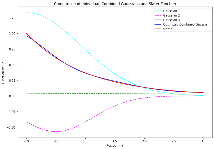
縮約ガウス関数 $\phi_\mathsf{blue}$ のパラメータは、スレーター型関数 $\phi_\mathsf{red}$ との二乗誤差を最小化することで最適化した

$$\phi_\mathsf{blue} = (1.33 e^{-0.59 r^2})_\mathsf{cyan}$$

$$+ (-0.57 e^{-1.28 r^2})_\mathsf{pink}$$

$$ + (0.04 e^{+0.06 r^2})_\mathsf{green}$$

import numpy as np
import matplotlib.pyplot as plt
from scipy.optimize import minimize

# Define Gaussian and Slater functions
def gaussian(r, coeff, alpha, center=0):
    return coeff * np.exp(-alpha * (r-center)**2)

def slater(r, coeff, alpha):
    return coeff * np.exp(-alpha * r)

# Define combined Gaussian function
def gaussian_combined(r, coeffs, alphas, centers):
    return sum(gaussian(r, coeff, alpha, center) for coeff, alpha, center in zip(coeffs, alphas, centers))

# Define the range for plotting
r_values = np.linspace(0, 3, 400)

# Parameters for the Slater function
alpha_slater = 1
coeff_slater = 1
slater_values = slater(r_values, coeff_slater, alpha_slater)

# Optimized parameters from previous steps
optimized_coeffs = [1.33, -0.57, 0.04]
optimized_alphas = [0.59, 1.28, -0.06]
centers = [0, 0.5, 1]

# Compute the individual Gaussian values with optimized parameters
gaussian_values_1 = gaussian(r_values, optimized_coeffs[0], optimized_alphas[0], centers[0])
gaussian_values_2 = gaussian(r_values, optimized_coeffs[1], optimized_alphas[1], centers[1])
gaussian_values_3 = gaussian(r_values, optimized_coeffs[2], optimized_alphas[2], centers[2])

# Compute the values for the optimized combined Gaussian functions
gaussian_optimized_values = gaussian_combined(r_values, optimized_coeffs, optimized_alphas, centers)

# Plotting
fig, ax = plt.subplots(figsize=(10, 7))

# Plot individual Gaussians
ax.plot(r_values, gaussian_values_1, label="Gaussian 1", color="cyan", linestyle="--")
ax.plot(r_values, gaussian_values_2, label="Gaussian 2", color="magenta", linestyle="--")
ax.plot(r_values, gaussian_values_3, label="Gaussian 3", color="green", linestyle="--")

# Plot the optimized combined Gaussian and Slater function
ax.plot(r_values, gaussian_optimized_values, label="Optimized Combined Gaussian", color="blue", linestyle="-")
ax.plot(r_values, slater_values, label="Slater", color="red", linestyle="-")

ax.set_xlabel("Position (r)")
ax.set_ylabel("Function Value")
ax.legend()
ax.set_title("Comparison of Individual, Combined Gaussians and Slater Function")

plt.tight_layout()
plt.show()

Conclusion

できた

量子化学教育

Posted : 23.10.25