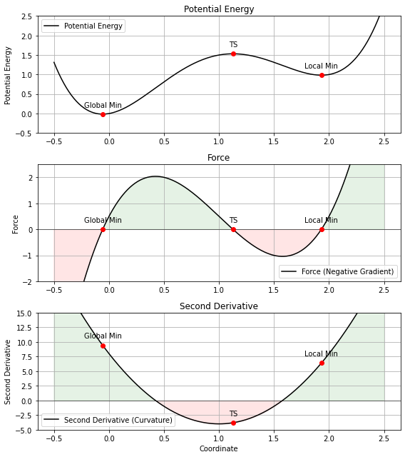
import numpy as np
import matplotlib.pyplot as plt
from scipy.optimize import fsolve

# Define a potential energy function (e.g., a simple polynomial)
def V(x):
    return x**4 - 4*x**3 + 4*x**2 + 0.5 * x

# Compute its first derivative (Force)
def dV(x):
    return 4*x**3 - 12*x**2 + 8*x + 0.5

# Compute its second derivative
def ddV(x):
    return 12*x**2 - 24*x + 8

# Define the function for which we want to find the roots (i.e., where the force is zero)
def roots_function(x):
    return dV(x)

# Compute the roots using fsolve with different initial guesses
roots = fsolve(roots_function, [-0.5, 0.5, 2.5])
roots = np.unique(np.round(roots, 5))  # Ensure the roots are unique
# Sort these roots based on the value of the potential function
sorted_roots = sorted(roots, key=lambda root: V(root))
global_min_x = sorted_roots[0]
local_min_x = sorted_roots[1]
ts_x = sorted_roots[2]

# Define the range for x
x = np.linspace(-0.5, 2.5, 400)

# Create the plots with an additional subplot for the second derivative
fig, (ax1, ax2, ax3) = plt.subplots(3, 1, figsize=(8, 9))

# Plot the potential energy function
ax1.plot(x, V(x), '-k', label='Potential Energy')
ax1.set_title("Potential Energy")
ax1.set_ylabel("Potential Energy")
ax1.set_ylim(-0.5,2.5)
ax1.grid(True)
ax1.legend()
# Annotate the Global Min, TS, and Local Min on the Potential energy curve
for x_val, label in zip([global_min_x, ts_x, local_min_x], ["Global Min", "TS", "Local Min"]):
    ax1.plot(x_val, V(x_val), 'ro')
    ax1.annotate(label, (x_val, V(x_val)), textcoords="offset points", xytext=(0,10), ha='center')

# Plot its first derivative (i.e., the force)
ax2.plot(x, dV(x), '-k', label='Force (Negative Gradient)')
ax2.axhline(0, color='black',linewidth=0.5)
ax2.set_title("Force")
ax2.set_ylabel("Force")
ax2.set_ylim(-2,2.5)
ax2.grid(True)
ax2.legend()
# Fill between the Force curve and x-axis
ax2.fill_between(x, dV(x), 0, where=(dV(x) > 0), color='green', alpha=0.1)
ax2.fill_between(x, dV(x), 0, where=(dV(x) < 0), color='red', alpha=0.1)
# Annotate the Global Min, TS, and Local Min on the Force curve
for x_val, label in zip([global_min_x, ts_x, local_min_x], ["Global Min", "TS", "Local Min"]):
    ax2.plot(x_val, dV(x_val), 'ro')
    ax2.annotate(label, (x_val, dV(x_val)), textcoords="offset points", xytext=(0,10), ha='center')

# Plot the second derivative
ax3.plot(x, ddV(x), '-k', label='Second Derivative (Curvature)')
ax3.axhline(0, color='black',linewidth=0.5)
ax3.set_title("Second Derivative")
ax3.set_xlabel("Coordinate")
ax3.set_ylabel("Second Derivative")
ax3.set_ylim(-5,15)
ax3.grid(True)
ax3.legend()
# Fill between the Second Derivative curve and x-axis
ax3.fill_between(x, ddV(x), 0, where=(ddV(x) > 0), color='green', alpha=0.1)
ax3.fill_between(x, ddV(x), 0, where=(ddV(x) < 0), color='red', alpha=0.1)
# Annotate the Global Min, TS, and Local Min on the Second Derivative curve
for x_val, label in zip([global_min_x, ts_x, local_min_x], ["Global Min", "TS", "Local Min"]):
    ax3.plot(x_val, ddV(x_val), 'ro')
    ax3.annotate(label, (x_val, ddV(x_val)), textcoords="offset points", xytext=(0,10), ha='center')

plt.tight_layout()
plt.show()