調和型関数 vs モース型関数：可視化して比較

Introduction

量子化学計算で振動解析をおこなったとき、高波数領域にある振動モード（O-H伸縮振動など）では、計算で予測される振動数が実験値と大きくズレてしまう
上記について、調和型関数 vs 非調和なモース型関数で比較しながら説明するための良い感じのグラフを描画したい

Method

調和型関数

形状: 対称なカタチ、放物線 $$ V_{\text{harmonic}}(r) = \frac{1}{2} k (r - r_0)^2 $$
- $k$ ：ばね定数
- $r_0$ ：平衡位置
固有値: 均等な間隔 $$ E_n = \left(n + \frac{1}{2}\right) \hbar \omega$$
$n = 0, 1, 2, \cdots$：量子数
$\omega = \sqrt{\frac{k}{m}}$：角振動数

モース型関数

形状: 非対称なカタチ $$V_{\text{Morse}}(r) = D_e \left(1 - \exp\left(-\alpha (r - r_e)\right)\right)^2$$
- $D_e$：井戸の深さ
- $\alpha$ ：関数の幅を決定するパラメータ
- $r_e$：平衡位置
固有値: だんだんと幅が狭まる $$E_n = \hbar \omega \left(n + \frac{1}{2}\right) - \frac{1}{4 D_e}\left(\hbar \omega \left(n + \frac{1}{2}\right)\right)^2$$
- $n = 0, 1, 2, \cdots$：量子数
- $\omega = \alpha \sqrt{\frac{2 D_e}{m}}$：角振動数

Results

import numpy as np
import matplotlib.pyplot as plt
from scipy.optimize import minimize

# Constants
hbar = 1
mass = 1

# Define the Morse potential function with offset
def morse_potential(r, De, alpha, re, offset):
    return De * (1 - np.exp(-alpha * (r - re)))**2 + offset

# Define the harmonic potential function with offset
def harmonic_potential(r, k, r0, offset):
    return 0.5 * k * (r - r0)**2 + offset

# Define function to plot eigenvalues with labels
def plot_eigenvalues_with_labels(r_values, potential_values, eigenvalues, color='blue'):
    for n, E in enumerate(eigenvalues):
        cross_points = np.where(potential_values < E)[0]
        if len(cross_points) > 0:
            start = cross_points[0]
            end = cross_points[-1]
            plt.hlines(E, r_values[start], r_values[end], colors=color, linestyles='--')
            label_x = r_values[end] + 0.1
            plt.text(label_x, E, f"n={n}", verticalalignment='center', color=color)

# Parameters provided
De = 5
alpha = 0.3
re = 3.5
morse_offset = 0

k = 1.0
r0 = 3.5
harmonic_offset = 0

# Define the error function with the restricted range for optimization
r_values = np.linspace(0, 10, 500)
r_min = r0 - 0.1
r_max = r0 + 0.1
mask = (r_values >= r_min) & (r_values <= r_max)
def error_function_restricted(params):
    De_new, alpha_new, re_new = params
    morse_new = morse_potential(r_values[mask], De_new, alpha_new, re_new, morse_offset)
    harmonic_new = harmonic_potential(r_values[mask], k, r0, harmonic_offset)
    error_potential = np.sum((morse_new - harmonic_new)**2)
    error_derivative = np.sum((np.gradient(morse_new) - np.gradient(harmonic_new))**2)
    return error_potential + error_derivative

# Optimize the parameters within the restricted range
result = minimize(error_function_restricted, [De, alpha, re], method='Nelder-Mead')
De_opt, alpha_opt, re_opt = result.x

# Calculate the potentials using the optimized parameters for the restricted range
morse_values_opt = morse_potential(r_values, De_opt, alpha_opt, re_opt, morse_offset)
harmonic_values = harmonic_potential(r_values, k, r0, harmonic_offset)

# Angular frequencies for the potentials
omega_harmonic = np.sqrt(k / mass)
omega_morse = alpha_opt * np.sqrt(2 * De_opt / mass)

# Eigenenergies
E_harmonic = [(n + 0.5) * hbar * omega_harmonic for n in range(5)]
E_morse = [hbar * omega_morse * (n + 0.5) - (hbar * omega_morse * (n + 0.5))**2 / (4 * De_opt) for n in range(5)]

# Plot the functions and eigenvalues with quantum number labels
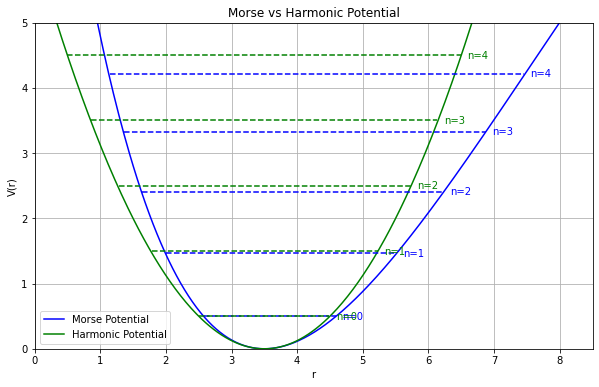
plt.figure(figsize=(10,6))
plt.plot(r_values, morse_values_opt, 'b', label='Morse Potential')
plt.plot(r_values, harmonic_values, 'g', label='Harmonic Potential')
plot_eigenvalues_with_labels(r_values, morse_values_opt, E_morse, color='blue')
plot_eigenvalues_with_labels(r_values, harmonic_values, E_harmonic, color='green')

plt.xlabel('r')
plt.ylabel('V(r)')
plt.xlim([0, 8.5])
plt.ylim([0, 5])
plt.legend()
plt.title('Morse vs Harmonic Potential')
plt.grid(True)
plt.show()

Conclusion

できた

量子化学教育

Posted : 23.10.26