


String method for finding the minimum energy path on PES
Introduction
- The String method1 is often used in computational chemistry to find minimum energy pathways (MEPs) on potential energy surfaces (PES).
- This method, used to analyze chemical reactions, provides a deeper understanding of the reaction pathways from reactants to products, making it a crucial tool in computational chemistry.
- In this note, as an example, I will present a simple Python code of the string method using the Muller-Brown potential2, often used to demonstrate path optimizations.
Code
- Here is a Python code for this demonstration.
import numpy as np
import matplotlib.pyplot as plt
# Parameters for the Muller-Brown potential
A = [-200, -100, -170, 15]
a = [-1, -1, -6.5, 0.7]
b = [0, 0, 11, 0.6]
c = [-10, -10, -6.5, 0.7]
x0 = [1, 0, -0.5, -1]
y0 = [0, 0.5, 1.5, 1]
# Function to calculate the potential energy
def muller_brown_potential(x, y):
z = 0
for i in range(4):
z += A[i] * np.exp(a[i]*(x-x0[i])**2 + b[i]*(x-x0[i])*(y-y0[i]) + c[i]*(y-y0[i])**2)
return z
# Function to calculate the gradient (force) of the potential
def muller_brown_gradient(x, y):
grad_x = 0
grad_y = 0
for i in range(4):
exp_term = np.exp(a[i]*(x-x0[i])**2 + b[i]*(x-x0[i])*(y-y0[i]) + c[i]*(y-y0[i])**2)
grad_x += exp_term * A[i] * (2*a[i]*(x-x0[i]) + b[i]*(y-y0[i]))
grad_y += exp_term * A[i] * (2*c[i]*(y-y0[i]) + b[i]*(x-x0[i]))
return np.array([grad_x, grad_y])
# Function to reparameterize the path to ensure equal spacing of points
def reparameterize(path, num_points):
# Calculate distances between consecutive points
distances = np.sqrt(np.sum(np.diff(path, axis=0)**2, axis=1))
# Calculate cumulative distances along the path
cumulative_distances = np.insert(np.cumsum(distances), 0, 0)
total_distance = cumulative_distances[-1]
# Generate new points with equal spacing
new_points = np.linspace(0, total_distance, num_points)
new_path = np.zeros((num_points, path.shape[1]))
for i in range(path.shape[1]):
new_path[:, i] = np.interp(new_points, cumulative_distances, path[:, i])
return new_path
# Function to optimize the path using the string method
def string_method(path, learning_rate, num_steps, num_points, interval):
paths = [np.copy(path)]
# Iteratively adjust the path
for step in range(num_steps):
new_path = [path[0]]
for i in range(1, len(path) - 1):
# Calculate gradient at the current point
grad = muller_brown_gradient(path[i][0], path[i][1])
# Update point position using gradient descent
new_point = path[i] - learning_rate * grad
new_path.append(new_point)
new_path.append(path[-1])
# Reparameterize the path to maintain equal spacing
path = reparameterize(np.array(new_path), num_points)
# Store the path at specified intervals
if step % interval == 0 or step == num_steps - 1:
paths.append(np.copy(path))
return paths
# Set initial path points
starting_point = np.array([-0.5, 1.5])
ending_point = np.array([0.6, 0.0])
initial_path = np.linspace(starting_point, ending_point, 10)
# Set parameters for the optimization
learning_rate = 0.0001
num_points = 15 # Number of points in the final path
interval = 15 # Interval for storing paths
num_steps = interval * 10 # Total number of optimization steps
# Optimize the path using the string method
paths = string_method(initial_path, learning_rate, num_steps, num_points, interval)
# Generate a grid of points to calculate the potential energy surface
x = np.linspace(-1.25, 1.0, 400)
y = np.linspace(-0.25, 1.75, 400)
X, Y = np.meshgrid(x, y)
Z = muller_brown_potential(X, Y)
plt.figure(figsize=(10, 8))
# Plot contour levels focusing on lower energy regions
contour_levels = np.linspace(Z.min(), Z.min() + 150, 50)
plt.contour(X, Y, Z, levels=contour_levels, cmap='Greys')
# Plot the optimized paths at each interval
colors = plt.cm.jet_r(np.linspace(0, 1, len(paths)))
for idx, path in enumerate(paths[:-1]):
plt.plot(path[:, 0], path[:, 1], marker='o', color=colors[idx], label=f'Step {idx*interval}')
# Display the gradient at each discrete point with arrows
for point in path:
grad = muller_brown_gradient(point[0], point[1])
plt.quiver(point[0], point[1], -grad[0], -grad[1], color=colors[idx], scale=5000, zorder=5)
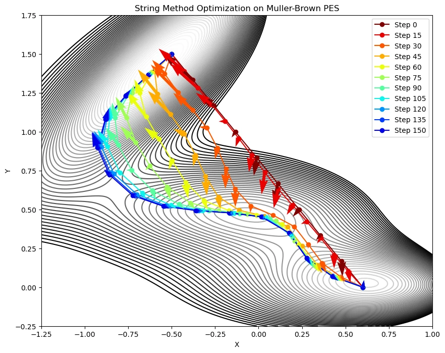
plt.title('String Method Optimization on Muller-Brown PES')
plt.xlabel('X')
plt.ylabel('Y')
plt.legend()
plt.show()- After executing the above Python code, the path optimization using the string method can be visualized in the following graph.
Muller-Brown potential
- This demonstration tries to find the minimum energy path connecting two points on the Muller-Brown (MB) potential.
- The MB potential is defined by a series of Gaussian functions as follows:
$$ V(x, y) = \sum_{i=1}^{4} A_i \exp \left( a_i (x - x_{0,i})^2 + b_i (x - x_{0,i})(y - y_{0,i}) + c_i (y - y_{0,i})^2 \right) $$
- The MB potential function is implemented as follows:
def muller_brown_potential(x, y):
    z = 0
    for i in range(4):
        z += A[i] * np.exp(a[i]*(x-x0[i])**2 + b[i]*(x-x0[i])*(y-y0[i]) + c[i]*(y-y0[i])**2)
return z- Here, $A$, $a$, $b$, $c$, $x_0$, and $y_0$ are parameters that define the potentials; in Python scripts, these parameters are defined as follows:
A = [-200, -100, -170, 15]
a = [-1, -1, -6.5, 0.7]
b = [0, 0, 11, 0.6]
c = [-10, -10, -6.5, 0.7]
x0 = [1, 0, -0.5, -1]
y0 = [0, 0.5, 1.5, 1]
Potential energy gradient
- To optimize the path, the gradient (or force) at each point must be calculated.
- The gradient of the potential $V$ is given by the partial derivatives with respect to $x$ and $y$.
$$ \nabla V(x, y) = \left( \frac{\partial V}{\partial x}, \frac{\partial V}{\partial y} \right) $$
- In the Python code, it is implemented as follows:
def muller_brown_gradient(x, y):
    grad_x = 0
    grad_y = 0
    for i in range(4):
        exp_term = np.exp(a[i]*(x-x0[i])**2 + b[i]*(x-x0[i])*(y-y0[i]) + c[i]*(y-y0[i])**2)
        grad_x += exp_term * A[i] * (2*a[i]*(x-x0[i]) + b[i]*(y-y0[i]))
        grad_y += exp_term * A[i] * (2*c[i]*(y-y0[i]) + b[i]*(x-x0[i]))
    return np.array([grad_x, grad_y])
String method
- The String method is a way to minimize energy by iteratively adjusting the pathway.
- The step-by-step details are as follows:
- Path initialization: Initialize the path between two points.
- Gradient Descent: Move each point on the path slightly toward the gradient.
- Reparameterization: Reposition the points on the path evenly.
- Iteration: Repeat the process until convergence.
- The path optimization function in the Python code is as follows:
def string_method(path, learning_rate, num_steps, num_points, interval):
    paths = [np.copy(path)]
    for step in range(num_steps):
        new_path = [path[0]]
        for i in range(1, len(path) - 1):
            grad = muller_brown_gradient(path[i][0], path[i][1])
            new_point = path[i] - learning_rate * grad
            new_path.append(new_point)
        new_path.append(path[-1])
        path = reparameterize(np.array(new_path), num_points)
        if step % interval == 0 or step == num_steps - 1:
            paths.append(np.copy(path))
    return paths
Visualization
- Plot the optimization of the path on the PES represented by the contour lines.
x = np.linspace(-1.25, 1.0, 400)
y = np.linspace(-0.25, 1.75, 400)
X, Y = np.meshgrid(x, y)
Z = muller_brown_potential(X, Y)

plt.figure(figsize=(10, 8))
contour_levels = np.linspace(Z.min(), Z.min() + 150, 50)
plt.contour(X, Y, Z, levels=contour_levels, cmap='Greys')

colors = plt.cm.jet_r(np.linspace(0, 1, len(paths)))
for idx, path in enumerate(paths[:-1]):
    plt.plot(path[:, 0], path[:, 1], marker='o', color=colors[idx], label=f'Step {idx*interval}')
    for point in path:
        grad = muller_brown_gradient(point[0], point[1])
        plt.quiver(point[0], point[1], -grad[0], -grad[1], color=colors[idx], scale=5000, zorder=5)

plt.title('String Method Optimization on Muller-Brown PES')
plt.xlabel('X')
plt.ylabel('Y')
plt.legend()
plt.show()
Conclusion
- The String method is simple to implement, as shown here.
- Combining this approach with quantum chemical calculations can also obtain the MEPs involved in various chemical reactions.
W. E, W. Ren, and E. Vanden-Eijnden, Phys. Rev. B, Vol. 66, p. 052301 (2002) doi: 10.1103/PhysRevB.66.052301 ↩︎
K. Müller and L. D. Brown, Theor. Chim. Acta, Vol. 53, p. 75 (1979) doi: 10.1007/BF00547608 ↩︎


