Nudged Elastic Band (NEB) 法で最小エネルギー経路を探索しよう
Nudged Elastic Band (NEB) 法
これは何か?
- NEB 法は、最小エネルギー経路の探索で使われる一般的な方法
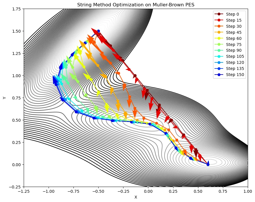
- 上の図は、MEP 探索手法の string 法を使ったときの経路変化だけど、NEB 法もだいたい同じような感じ
計算手順は?
- 始状態と終状態の間に複数の中間点(image と呼ぶ)を作る
- それぞれの image で量子化学計算を実行して系に掛かる力 Fを求める
- 各 image について、反応経路の方向と直交する力 $F_\perp$ の方向に動かす
- image 同士には「バネ」のような力が掛かっていて、離れすぎずない・近づきすぎない
Gaussian で使える?
- 現在のバージョンには実装されていない(将来的にはわからない)
- HPC システムズ(株)が開発・販売している Reaction Plus
(学術:80 万円、商用:200 万円)というソフトウェアと Gaussian を組み合わせると NEB 計算ができる
- ただし、Reaction plus Pro は1台のパソコンしかインストールできないので、スパコンでは使えない
- Atomic Simulation Environment (ASE)
という Python のモジュールを使うと、ちょっと手間は掛かるけれど、無料で NEB 計算ができる
ASE を使って NEB 計算
ASE のインストール
- Python 環境が整っていれば、ASE のインストールは
pipコマンドだけで完了
pip3 install --upgrade --user ase
NEB 計算を実行するための Python スクリプト
- 複雑そうに見えますが、設定する部分は多くありません
- Python と ASE のインストールさえ上手くいけば、比較的お手軽に、NEB 計算ができます
#!/usr/bin/python3

# ===== 設定 =====

# 始状態の構造(xyz 形式)
geom_of_reactant = "open.xyz"
# 終状態の構造(xyz 形式)
geom_of_product  = "closed.xyz"
# NEB 計算の離散点(images)の個数
numb_of_nodes = 18
# 計算の収束条件
convergence = 0.4

# 計算方法
gaussian_method = "B3LYP"
# 基底関数
gaussian_basis = "6-31G(d)"
# 電荷
gaussian_charge = 0
# スピン多重度
gaussian_mult = 1

# ===== 必要な設定はここまで =====

import os

from ase import Atoms
from ase.io import read,write
from ase.calculators.gaussian import Gaussian
from ase.build.rotate import minimize_rotation_and_translation
from ase.optimize import BFGS
from ase.neb import NEB

atoms_reac = read(geom_of_reactant)
atoms_prod = read(geom_of_product)

if not os.path.exists("neb"):
    os.mkdir("neb")

images = []
for n in range(numb_of_nodes):
    if n < (numb_of_nodes // 2):
        image = atoms_reac.copy()
    else:
        image = atoms_prod.copy()
    minimize_rotation_and_translation(atoms_reac, image)
    image.calc = Gaussian(label = 'neb/Gaussian', mem = "19200MB", chk = "Gaussian.chk", save = None,
                          method = gaussian_method, basis = gaussian_basis, charge = gaussian_charge, mult = gaussian_mult)
    images.append(image)

neb = NEB(images)
neb.interpolate()

pote_old = [image.get_potential_energy() for image in images]

path_opt = BFGS(neb, trajectory = 'neb.traj', logfile = 'neb.log')
path_opt.run(fmax = convergence)

pote_new = [image.get_potential_energy() for image in images]

with open("neb.dat", 'w') as fw:
    for n in range(numb_of_nodes):
        fw.write(f"{n:2d}  {pote_old[n]:20.10f}  {pote_new[n]:20.10f}\n")

if os.path.exists("neb.xyz"):
    os.remove("neb.xyz")
for n in range(numb_of_nodes):
    write("neb.xyz", images[n], append = True)
- 分子研などのスパコンで実行する場合には、下記のようなジョブファイルが必要
#!/bin/sh
#PBS -l select=1:ncpus=16:mpiprocs=1:ompthreads=16
#PBS -l walltime=2:00:00

NCPUS=16
FILE="neb.py"

if [ ! -z "${PBS_O_WORKDIR}" ]; then
  cd "${PBS_O_WORKDIR}"
  WORK=/lwork/users/${USER}/${PBS_JOBID}/gaussian
else
  WORK=/gwork/users/${USER}/tmp.$$
fi

if [ ! -d ${WORK} ]; then
  mkdir ${WORK}
fi

. /apl/gaussian/16c02/g16/bsd/g16.profile
export LANG=C
export GAUSS_SCRDIR=${WORK}

export GAUSS_CDEF=`/apl/gaussian/16c02/rccs/cpu.pl -n $NCPUS`

python ${FILE}

if [ -d ${WORK} ]; then
  /bin/rm -rf ${WORK}
fi
exit 0
Gaussian + ASE を用いた NEB 計算の例
NEB 計算のログファイル
      Step     Time          Energy          fmax
BFGS:    0 06:31:49   -86679.654521         4.536103
BFGS:    1 06:32:55   -86680.216141         1.420071
BFGS:    2 06:34:02   -86680.359441         0.905582
BFGS:    3 06:35:07   -86680.486887         1.321789
BFGS:    4 06:36:12   -86680.588479         1.304590
BFGS:    5 06:37:15   -86680.690182         0.843390
BFGS:    6 06:38:22   -86680.752385         0.582411
BFGS:    7 06:39:31   -86680.774994         0.406031
BFGS:    8 06:40:38   -86680.785722         0.367132
NEB 計算の出力ファイル
 0     -86680.2025041622     -86680.2025041622
 1     -86680.1578995303     -86680.7857217171
 2     -86680.0664118573     -86680.8168607946
 3     -86679.9496488883     -86680.8351969150
 4     -86679.8306700962     -86680.8485386575
 5     -86679.7316475903     -86680.8564389393
 6     -86679.6697226391     -86680.8581124395
 7     -86679.6545207262     -86680.8520794031
 8     -86679.6850690445     -86680.8361838720
 9     -86679.7481412277     -86680.8076657952
10     -86680.1616693957     -86681.0704973074
11     -86680.5426617259     -86681.2701192190
12     -86680.9831582823     -86681.5302249667
13     -86681.4684143033     -86681.8561311111
14     -86681.9808898738     -86682.2407194259
15     -86682.4964852297     -86682.6580351468
16     -86682.9729010877     -86683.0511849800
17     -86683.2444728972     -86683.2444728972
NEB 計算の結果


